glTF-Tutorials
| Previous: Simple Animation | Table of Contents | Next: Simple Meshes |
Animations
As shown in the Simple Animation example, an animation can be used to describe how the translation, rotation, or scale properties of nodes change over time.
The following is another example of an animation. This time, the animation contains two channels. One animates the translation, and the other animates the rotation of a node:
  "animations": [
    {
      "samplers" : [
        {
          "input" : 2,
          "interpolation" : "LINEAR",
          "output" : 3
        },
        {
          "input" : 2,
          "interpolation" : "LINEAR",
          "output" : 4
        }
      ],
      "channels" : [
        {
          "sampler" : 0,
          "target" : {
            "node" : 0,
            "path" : "rotation"
          }
        },
        {
          "sampler" : 1,
          "target" : {
            "node" : 0,
            "path" : "translation"
          }
        }
      ]
    }
  ],
Animation samplers
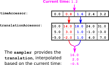
The samplers array contains animation.sampler objects that define how the values that are provided by the accessors have to be interpolated between the key frames, as shown in Image 7a.
In order to compute the value of the translation for the current animation time, the following algorithm can be used:
- Let the current animation time be given as
currentTime. -
Compute the next smaller and the next larger element of the times accessor:
previousTime= The largest element from the times accessor that is smaller than thecurrentTimenextTime= The smallest element from the times accessor that is larger than thecurrentTime -
Obtain the elements from the translations accessor that correspond to these times:
previousTranslation= The element from the translations accessor that corresponds to thepreviousTimenextTranslation= The element from the translations accessor that corresponds to thenextTime -
Compute the interpolation value. This is a value between 0.0 and 1.0 that describes the relative position of the
currentTime, between thepreviousTimeand thenextTime:interpolationValue = (currentTime - previousTime) / (nextTime - previousTime) -
Use the interpolation value to compute the translation for the current time:
currentTranslation = previousTranslation + interpolationValue * (nextTranslation - previousTranslation)
Example:
Imagine the currentTime is 1.2. The next smaller element from the times accessor is 0.8. The next larger element is 1.6. So
previousTime = 0.8
nextTime     = 1.6
The corresponding values from the translations accessor can be looked up:
previousTranslation = (14.0, 3.0, -2.0)
nextTranslation     = (18.0, 1.0,  1.0)
The interpolation value can be computed:
interpolationValue = (currentTime - previousTime) / (nextTime - previousTime)
                   = (1.2 - 0.8) / (1.6 - 0.8)
                   = 0.4 / 0.8
                   = 0.5
From the interpolation value, the current translation can be computed:
currentTranslation = previousTranslation + interpolationValue * (nextTranslation - previousTranslation)
                   = (14.0, 3.0, -2.0) + 0.5 * ( (18.0, 1.0,  1.0) - (14.0, 3.0, -2.0) )
                   = (14.0, 3.0, -2.0) + 0.5 * (4.0, -2.0, 3.0)
                   = (16.0, 2.0, -0.5)
So when the current time is 1.2, then the translation of the node is (16.0, 2.0, -0.5).
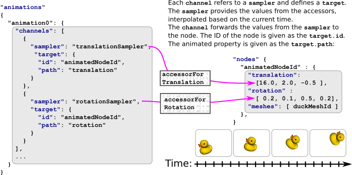
Animation channels
The animations contain an array of animation.channel objects. The channels establish the connection between the input, which is the value that is computed from the sampler, and the output, which is the animated node property. Therefore, each channel refers to one sampler, using the index of the sampler, and contains an animation.channel.target. The target refers to a node, using the index of the node, and contains a path that defines the property of the node that should be animated. The value from the sampler will be written into this property.
In the example above, there are two channels for the animation. Both refer to the same node. The path of the first channel refers to the translation of the node, and the path of the second channel refers to the rotation of the node. So all objects (meshes) that are attached to the node will be translated and rotated by the animation, as shown in Image 7b.
Interpolation
The above example only covers LINEAR interpolation. Animations in a glTF asset can use three interpolation modes :
STEPLINEARCUBICSPLINE
Step
The STEP interpolation is not really an interpolation mode, it makes objects jump from keyframe to keyframe without any sort of interpolation. When a sampler defines a step interpolation, just apply the transformation from the keyframe corresponding to previousTime.
Linear
Linear interpolation exactly corresponds to the above example. The general case is :
Calculate the interpolationValue:
interpolationValue = (currentTime - previousTime) / (nextTime - previousTime)
For scalar and vector types, use a linear interpolation (generally called lerp in mathematics libraries). Here’s a “pseudo code” implementation for reference
    Point lerp(previousPoint, nextPoint, interpolationValue)
        return previousPoint + interpolationValue * (nextPoint - previousPoint)
In the case of rotations expressed as quaternions, you need to perform a spherical linear interpolation (slerp) between the previous and next values:
    Quat slerp(previousQuat, nextQuat, interpolationValue)
        var dotProduct = dot(previousQuat, nextQuat)

        //make sure we take the shortest path in case dot Product is negative
        if(dotProduct < 0.0)
            nextQuat = -nextQuat
            dotProduct = -dotProduct

        //if the two quaternions are too close to each other, just linear interpolate between the 4D vector
        if(dotProduct > 0.9995)
            return normalize(previousQuat + interpolationValue(nextQuat - previousQuat))

        //perform the spherical linear interpolation
        var theta_0 = acos(dotProduct)
        var theta = interpolationValue * theta_0
        var sin_theta = sin(theta)
        var sin_theta_0 = sin(theta_0)

        var scalePreviousQuat = cos(theta) - dotproduct * sin_theta / sin_theta_0
        var scaleNextQuat = sin_theta / sin_theta_0
        return scalePreviousQuat * previousQuat + scaleNextQuat * nextQuat
This example implementation is inspired from this Wikipedia article
Cubic Spline interpolation
Cubic spline interpolation needs more data than just the previous and next keyframe time and values, it also need for each keyframe a couple of tangent vectors that act to smooth out the curve around the keyframe points.
These tangent are stored in the animation channel. For each keyframe described by the animation sampler, the animation channel contains 3 elements :
- The input tangent of the keyframe
- The keyframe value
- The output tangent
The input and output tangents are normalized vectors that will need to be scaled by the duration of the keyframe, we call that the deltaTime
deltaTime = nextTime - previousTime
To calculate the value for currentTime, you will need to fetch from the animation channel :
- The output tangent direction of
previousTimekeyframe - The value of
previousTimekeyframe - The value of
nextTimekeyframe - The input tangent direction of
nextTimekeyframe
note: the input tangent of the first keyframe and the output tangent of the last keyframe are totally ignored
To calculate the actual tangents of the keyframe, you need to multiply the direction vectors you got from the channel by deltaTime
    previousTangent = deltaTime * previousOutputTangent
    nextTangent = deltaTime * nextInputTangent
The mathematical function is described in the Appendix C of the glTF 2.0 specification.
Here’s a corresponding pseudocode snippet :
    Point cubicSpline(previousPoint, previousTangent, nextPoint, nextTangent, interpolationValue)
        t = interpolationValue
        t2 = t * t
        t3 = t2 * t

        return (2 * t3 - 3 * t2 + 1) * previousPoint + (t3 - 2 * t2 + t) * previousTangent + (-2 * t3 + 3 * t2) * nextPoint + (t3 - t2) * nextTangent;
| Previous: Simple Animation | Table of Contents | Next: Simple Meshes |